Click here to download the data file for this tutorial.

We are not always lucky to have our data neatly laid out in rows and columns. Sometimes, our data come in as a formatted report and we need to find a way to massage the data before it can be loaded into a data model.

This tutorial will walk you through some common techniques that are useful for this scenario.

Step 1 – Connect to the data set

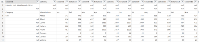
In Excel, go to Power Query->From File->From Excel then navigate to the folder where you saved the formatted Excel report. Then in the Power Query navigator find the Sheet1, right click on it and select “Edit”

You should see something in your Power Query window that looks like this:

Step 2 – Massage the data

1. Right click on the first cell in the first column of the data set, then select Text Filters->Does Not Equal

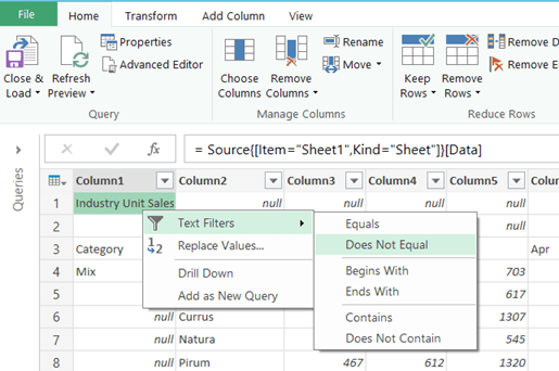
This allows us to quickly remove non-relevant data from our data set.

Typically, a formatted report will have things like comments, totals/sub totals or empty cells that need to be removed.

1. Now, find a “Null” value in column3 and filter it out the same way as above (Text Filters->Does Not Equal).

    

2. Click on “Use First Row as Headers” in the Ribbon

    

3. Now, note how the Category Value is only populated for the first record, we need make sure that every cell in that column is properly filled out.

    

   

    

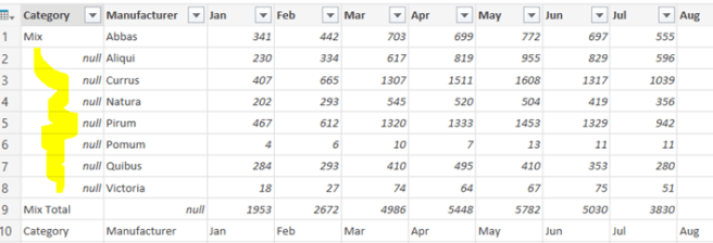
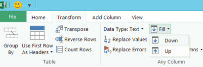
   Luckily, in Power Query it is easy to do. Click on the first cell in the Category column and then click on the Transform tab in the ribbon and select Fill->Down button

    

   

   You now should see that every cell in the Category column is populated.

    

4. Now we need to filter out other rows that contain either totals or not relevant information. Use the technique we described above to filter out rows in the Category column that have a word Total or Category in them. (hint, after you filter out a value, you can click on the Gear icon in the Applied Steps pane on the right and make changes if necessary, for example, after you found and filtered out “Mix Total” you can click on the gear icon for that step and change the filter condition from “Mix total” to just “total” which will take care of all cells with totals in them)

    

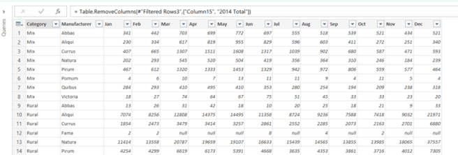
5. We also have some columns that we don’t want in our data set, therefore, click on Chose Columns in the Home tab of the ribbon and unselect “Column15” and “2014 Total“.

    

Step 3 – Unpivot columns

At this point we have filtered out all the unnecessary data from our data set, however, our data are still not laid out in the best format for consuming it in our model.

Having sales data in a separate column for each month makes sense in a report layout but if we went to load it into a Power Pivot model, we may want to massage it even more.

Shift-click the columns that contain the month names in them to select them and then click on Transform->Unpivot columns in the Power Query ribbon. Your data should now look like this:

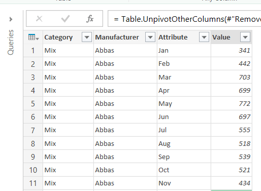
The month name was moved into an Attribute column, and the sales values into the Value column. Let’s rename these new columns into something a little bit more meaningful. The Attribute column should be named Month and the Value column – Units.

You can now click on Close & Load and build a simple pivot table report to do some analysis.