Power BI Tutorial: UnPivot Feature

It’s common that data is laid out across columns in Excel for reporting purposes. E.g. Revenue for each product is laid out across the columns in excel for each month. However this may not work well as a data source. Power Query provides Unpivot option to solve this issue.

Sample workbook can be downloaded here.

Here are the steps to unpivot data

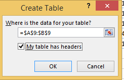
1. Insert a table by highlighting data in Excel. Click on Insert in the ribbon. Select Table and click OK

   

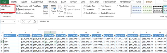
2. Rename the table, by highlighting the newly created table. Click on Design in the ribbon and rename the table to “Sales”

   

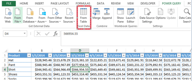
3. To create a Power Query, click on a cell in the Sales table. Click on Power Query in the ribbon, select “From Table”. This opens up Power Query editor window

   

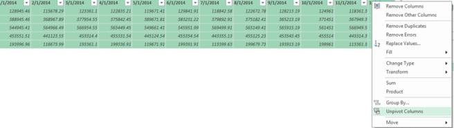
4. Highlight all the date columns, 1/1/2014 through 12/1/2014. Right click and select Unpivot Columns option

   

5. This unpivots the data

   

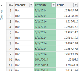
6. Rename Attribute column by highlighting it and right click to select Rename. Rename it to “Date”
7. Rename Value column by highlighting it and right click to select Rename. Rename it to “Revenue”

   

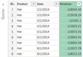
8. Click on “Close & Load” to load the data into Excel worksheet or the data model