Click Here to download this Tutorial file

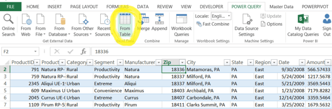
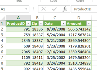
Very often our analysis starts with a flat data set that contains all of the pertinent columns in a single table that looks like the one above.

As we can see, we can analyze this data using three different lenses or dimensions:

1. Product
2. Geography
3. Date

Unfortunately, if we create a Pivot Table on top of that data set, the end result does not look particular user friendly as it essentially presents us with a flat list of all fields available for pivoting:

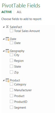
In this tutorial, we will learn how to massage the data using Power Query so that we can build a more user friendly model that looks like this:

Step 1 – Data preparation

The first thing to do is to load our data set into a Power Query environment so we can start massaging it. In our case, the dataset is contained in an Excel Table, so we can quickly create a Power Query on top of it by clicking Power Query->From Table

Now, in Power Query window, let’s make sure that all of our columns have a correct data type associated with them:

• Set the Date field to be Date
• Set the Amount field to be a Decimal Number
• Set Product ID to be a Whole Number

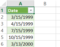
Here is a screen shot for how to change the Date data type

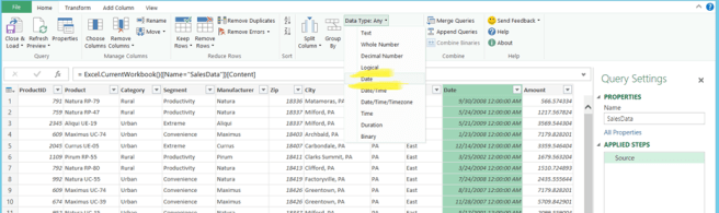
Click on Close & Load to load the results of this Power Query into a new tab in Excel

Step 2 – Create Product Dimension

Now that our data is properly formatted we are ready to create our dimensions. Let’s reuse the query we just made by right clicking it and choosing Duplicate option

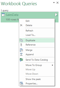
Now in our Workbook Queries pane we should have two entries

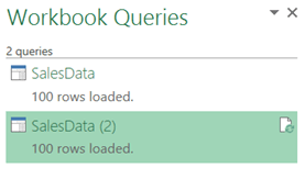
Double click on SalesData(2) and rename the new query as Product

Now let’s click on Choose Columns and uncheck those entries that don’t have anything to do with Products and click OK

The next step is to remove duplicate records by clicking on Product ID and then Remove Duplicate

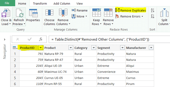
We now have a list of all unique Products in our data set. Click Close & Load to load the results of this Power Query into a new worksheet.

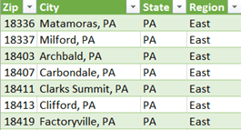
Step 3 – Geography and Date Dimensions

Now you can repeat these step by filtering out Geography only attributes to create a Geography dimension and the Date to create a Date Dimension, when you are done you should have two additional worksheets that look like this for Geography

And this for Date

My naming convention for worksheets is the following:

Step 4 – Create Fact Table

Let’s remove all unnecessary fields from our original data set now that we have moved them into separate dimensions:

1. Duplicate the SalesData Power Query again and rename the new one to say SalesFact
2. Remove all fields other than what we need to link back to our dimensions and let’s also keep our measure (Amount)

   

3. Close & Load

   

Step 5 – Power Pivot

Now that we have our data cleaned up and broken into Product, Geography and Date dimensions as well as a SalesFact fact table, we are ready to create our model. The default behavior of Close & Load option of Power Query is to load its results into a new Excel worksheet, we created our first Power Query (SalesData) we could have chosen to load the data into either Excel Worksheet or a Power Pivot Model by choosing Add This Data to the Data Model option (clicking on Only Create Connection tells Power Query not to load data into a worksheet)

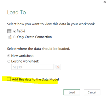
Since we did not use that option in the beginning, we have to right click on the Power Queries we want to add to our model and click on Load To… option

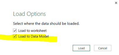
Now we can select Load to Data Model option to add the results of the Power Query to our Power Pivot Model

Let’s do this for the following Power Queries:

• Product
• Geography
• Date
• SalesFact

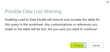
If you get a warning message that looks like this, please click Continue

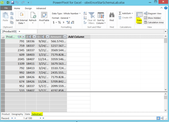
If we click on Power Pivot -> Manage we should see all of our tables there (click on Home->Diagram View to see all of them at the same time)

We can link our SalesFact table with dimensions by dragging a dropping ProductID, Zip and Date to their respective fields in respective dimensions. After you are done, the model should look like this:

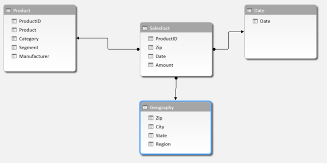
This layout, with a fact table in the middle and dimension tables around it, looks like a star (hence the name Star Schema)

The final step is to enhance our Fact table by hiding the unnecessary columns and creating a Total Sales calculation. In order to do that, make sure that you are in a Home->Data View and also make sure you have SalesFact table selected

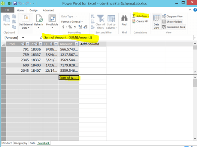
Click on Amount column then AutoSum. It should create a new calculation that is by default named Sum of Amount

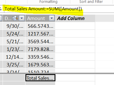
Click on the new calc and then rename ti in the Formula field above to say Total Sales Amount

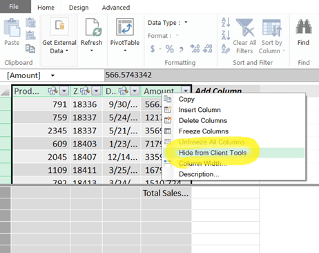
Now, let’s hide all columns in our fact table and our model is ready for analysis – shift click all columns in the SalesFact table to select them then right click and pick Hide from Client Tools.

Step 6 – Analysis

Let’s click on Home->Pivot Table in the Power Pivot window to create a new pivot table (pick New Worksheet option when prompted). Because we loaded our Power Queries both in worksheet and the power pivot model, we will see some duplication of table names, but if we had selected to load our Power Queries into a Data Model only (you can go and do that now if you want), our new model should look like this

As we can see this is a much more user friendly layout as all the data attributes are grouped in the appropriate buckets. This model is also ready to start meshing with other data sets. For example, if we were to purchase some 3^rd party data for demographics by zip code, all we would need to do to enhance our existing model with that data would be to add demographics data to Power Pivot and then link it to our Geography dimension by Zip Code.